
Build a Realtime Recommendation Engine: Part 1
Preface In today’s world, user experience is paramount. It’s no longer about basic CRUD, just ...
Learn more

This is part 2 of a two-part series on recommendations using Dgraph. Check our part 1 here.
In the last post, we looked at how many applications and web apps no longer present static data, but rather generate interesting recommendations to users. There’s a whole field of theory and practice in recommendation engines that we touched on, talking about content-based (based on properties of objects) and collaborative (based on similar users) filtering techniques based on a chapter from Stanford MOOC Minning Massive Datasets.
We dug deeper into content-based filtering and showed how Jaccard distance and Cosine distance can be encoded directly in Dgraph queries using Dgraph’s variables and math functions.
This time we’ll look into collaborative filtering and hybrid recommendations in Dgraph queries. Then we’ll look at how to build a real-time scalable recommendation engine for big graphs.
To start with, we’ll continue with our movie data from last time and then start looking at recommendations over Stack Exchange data. We’ll keep it small in this post and use Lifehacks data, but watch out for upcoming posts on loading all of Stack Overflow (2 Billion edges) into Dgraph and running the website and a recommendation engine with Dgraph as the backend.
Content-based filtering measures the similarity of objects based on their properties. Rather than trying to find similar items, collaborative filtering works by finding similar users and then recommending items that similar users have rated highly. In the movie example from part 1, for a given user we first find the set of users that are similar, find movies those users rated highly and recommend some that our user hasn’t seen.
Let’s say we are trying to recommend movies to Bob. If Bob and Alice have rated a movie highly and they do this repeatedly for many movies, they are similar. The more movies they have in common this way, the more similar Bob and Alice are. Once we have more similar users like Alice, we need to find those movies that these users have rated highly. We then remove the movies that Bob has seen, leaving movies we should recommend to Bob.
If we represent the movies that user $U_i$ and user $U_j$ have in common as
$$M_{(u_i,u_j)}$$
and write $R_{U_i}$ for a user’s rating function, then we can represent a distance (or similarity) score between two users as an average of their scores for the movies they both rated.

This is how the query would look in Dgraph.
{
  var(func: uid(2)) {                             # 1
    a as math(1)
    seen as rated @facets(r as rating) {  # 2
      ~rated @facets(sr as rating) {      # 3
        user_score as math((sr + r)/a)    # 4
      }
    }
  }

  var(func: uid(user_score), first:30, orderdesc: val(user_score)) {  # 5
    norm as math(1)
    rated @filter(not uid(seen)) @facets(ur as rating) {           # 6
      fscore as math(ur/norm)                                      # 7
    }
  }

  Recommendation(func: uid(fscore), orderdesc: val(fscore), first: 10) { # 8
    name
  }
}
Note that this query is slightly different from the formula in MOOC chapter, because although we can write cosine distance for content-based filtering directly in the query language, the language does not yet support cosine distance when it involves more than 1 traversal. However, this can be tackled by retrieving the subgraph from Dgraph, doing the computation and writing the similarity scores back to Dgraph for further processing.
Let us look at what different parts of the query do.
Output:
{
  "Recommendation": [
    {
      "name": "Hercules (1997)"
    },
    {
      "name": "How to Be a Player (1997)"
    },
    {
      "name": "Othello (1995)"
    },
    {
      "name": "U Turn (1997)"
    },
    {
      "name": "Edge, The (1997)"
    },
    {
      "name": "Arrival, The (1996)"
    },
    {
      "name": "Outlaw, The (1943)"
    },
    {
      "name": "Con Air (1997)"
    },
    {
      "name": "As Good As It Gets (1997)"
    },
    {
      "name": "From Dusk Till Dawn (1996)"
    }
  ]
}
Let’s make an improvement. Consider the case when user A rated movie-a 1, user B rated movie-a 5, user A rated movie-b 3 and user C rated movie-b 3. Based on the average score for common movies, both user B and C will have a score of 3. But intuitively, we can say that user C is more similar to A than B. One way to avoid this would be by considering only the good ratings which we can define as >= 3.
So we can add a filter when we’re getting the ratings as follows:
# Collaborative filtering
{
  var(func: uid(2)) {  # 1
    a as math(1)
    seen as rated @facets(r as rating) @facets(ge(rating, 3)) { # 2
      ~rated @facets(sr as rating) @facets(ge(rating, 3)) {     # 3
        user_score as math((sr + r)/a) # 4
      }
    }
  }

  var(func: uid(user_score), first:30, orderdesc: val(user_score)) { # 5
    norm as math(1)
    rated @filter(not uid(seen)) @facets(ur as rating) {          # 6
      fscore as math(ur/norm) # 7
    }
  }

  Recommendation(func: uid(fscore), orderdesc: val(fscore), first: 10) { # 8
    name
  }
}
Output:
{
  "Recommendation": [
    {
      "name": "Thinner (1996)"
    },
    {
      "name": "Tales from the Hood (1995)"
    },
    {
      "name": "Michael (1996)"
    },
    {
      "name": "Hour of the Pig, The (1993)"
    },
    {
      "name": "Basic Instinct (1992)"
    },
    {
      "name": "Wild Bunch, The (1969)"
    },
    {
      "name": "Bound (1996)"
    },
    {
      "name": "Richard III (1995)"
    },
    {
      "name": "Spitfire Grill, The (1996)"
    },
    {
      "name": "Garden of Finzi-Contini, The (Giardino dei Finzi-Contini, Il) (1970)"
    }
  ]
}
Let’s try and test how well this is working. We don’t have any live users to test on, but one measure can be how well it predicts the known data. We removed the following 5 movies that user 2 rated as 5 and ran the query to predict the ratings.
        {
          "_uid_": "0x30e5d",
          "name": "Secrets & Lies (1996)"
        },
        {
          "_uid_": "0x30e6e",
          "name": "L.A. Confidential (1997)"
        },
        {
          "_uid_": "0x30e77",
          "name": "Wings of the Dove, The (1997)"
        },
        {
          "_uid_": "0x30e79",
          "name": "Titanic (1997)"
        },
        {
          "_uid_": "0x30e7c",
          "name": "As Good As It Gets (1997)"
        }
The predicted ratings are:
        {
          "name": "Secrets & Lies (1996)",
          "var(fscore)": 5
        },
        {
          "name": "L.A. Confidential (1997)",
          "var(fscore)": 3
        },
        {
          "name": "Wings of the Dove, The (1997)",
          "var(fscore)": 5
        },
        {
          "name": "Titanic (1997)",
          "var(fscore)": 3.833333
        },
        {
          "name": "As Good As It Gets (1997)",
          "var(fscore)": 4.666667
        }
So 2 of the movies got 5 rating, one got 4.66, one 3.83, and one 3. Not bad for a single query!
Let’s tweak it some more. If the ratings by two users vary too, much they might not be as similar. For example, taking a straight average, ratings of 3 and 3 by the two users look the same as 5 and 1. So lets penalize each user by the difference in rating — as the rating difference grows the penalty increases.
In the query below we multiply the average by:
$$1 - {(\frac{sr-r}{5*a})}^2$$
If the difference between ratings is small, the multiple will be closer to 1. If the difference is larger, the multiple will be closer to 0, reducing the user’s similarity.
{
  var(func: uid(2)) {  # 1
    a as math(1)
    seen as rated @facets(r as rating) @facets(ge(rating, 3)) { # 2
      ~rated @facets(sr as rating) @facets(ge(rating, 3)) {     # 3
        user_score as math(
        (sr + r)/a *
        (1 -  pow((sr-r)/(5*a),
        2))) # 4
      }
    }
  }

  var(func: uid(user_score), first:30, orderdesc: val(user_score)) { #5
    norm as math(1)
    rated @filter(not uid(seen)) @facets(ur as rating) { # 6
      fscore as math(ur/norm) # 7
    }
  }

  Recommendation(func: uid(fscore), orderdesc: val(fscore), first: 10) { # 8
    val(fscore)
    name
  }
}
Predicated ratings for the ones that were removed from the dataset are:
        {
            "name": "Secrets & Lies (1996)",
            "var(fscore)": 5.0
        },
        {
            "name": "L.A. Confidential (1997)",
            "var(fscore)": 2.75
        },
        {
            "name": "Wings of the Dove, The (1997)",
            "var(fscore)": 5.0
        },
        {
            "name": "Titanic (1997)",
            "var(fscore)": 4.0
        },
        {
            "name": "As Good As It Gets (1997)",
            "var(fscore)": 4.666667
        },
The scores got closer to the removed actual scores, probably indicating that we removed some users from the similar users who didn’t vote highly for this movie. ‘‘L.A. Confidential’’ was a bit of an outlier, going back slightly, indicating that we removed some users who enjoyed this one.
Content-based filtering found similar movies, based on a given movie. Collaborative filtering found similar users and gave a recommendation of movies the similar users rated highly.
Hybrid filtering is when we combine the collaborative and content-based approaches into a single recommendation algorithm.
For our hybrid filtering, we’ll assign a score to each genre as the number of movies watched by user 2 in that genre. Then, after we’ve found the similar users, we’ll give a boost to the ratings of movies based on the genres that user 2 watches most. That’s collaborative filtering to get the similar users and the movies they enjoy, and then content-based filtering to help order those movies based on genres.
Warning
Query syntax and features has changed in v1.0 release. For the latest syntax and features, visit link to docs.
{
  var(func: uid(2)) {  # 1
    rated @groupby(genre) {
      gc as count(_uid_)
    }

    a as math(1)
    seen as rated @facets(r as rating) @facets(ge(rating, 3)) { # 2
      ~rated @facets(sr as rating) @facets(ge(rating, 3)) {   # 3
        user_score as math((sr + r)/a) # 4
      }
    }
  }

  var(func: uid(user_score), first:30, orderdesc: val(user_score)) { #5
    norm as math(1)
    rated @filter(not uid(seen)) @facets(ur as rating) { # 6
      genre {
        q as math(gc)   # 6.1
      }
      x as sum(val(q))  # 6.2
      fscore as math((1+(x/100))*ur/norm) # 7
    }
  }

  Recommendation(func: uid(fscore), orderdesc: val(fscore), first: 10) { # 8
    val(fscore)
    name
  }
}
This time, at step #1 the query gets a count of how many times our user has rated movies in each genre using Dgraph’s groupby, so gc will relate genres to number of movies rated in that genre. Then, before calculating the score for each movie at step #7, the query gives each genre in the movie a score, step 6.1, and sums a total score, step 6.2. At step #7 each movie’s average score is multiplied by $1+\frac{x}{100}$.
If a movie contains genres our user doesn’t watch so much, $\frac{x}{100}$ will be small and the movie won’t get much of a boost. If it contains genres our user often rates movies of, then $x$ will be larger and thus $1+\frac{x}{100}$ will give a bigger bonus.
Output:
{
    "Recommendation": [
        {
            "name": "Bound (1996)",
            "var(fscore)": 8.15
        },
        {
            "name": "Wings of the Dove, The (1997)",
            "var(fscore)": 7.75
        },
        {
            "name": "Kiss the Girls (1997)",
            "var(fscore)": 7.45
        },
        {
            "name": "Legends of the Fall (1994)",
            "var(fscore)": 7.4
        },
        {
            "name": "Jane Eyre (1996)",
            "var(fscore)": 7.25
        },
        {
            "name": "Crying Game, The (1992)",
            "var(fscore)": 7.065
        },
        {
            "name": "To Catch a Thief (1955)",
            "var(fscore)": 6.95
        },
        {
            "name": "American President, The (1995)",
            "var(fscore)": 6.857143
        },
        {
            "name": "Sirens (1994)",
            "var(fscore)": 6.813333
        },
        {
            "name": "As Good As It Gets (1997)",
            "var(fscore)": 6.813333
        }
    ]
}
With the collaborative filtering queries, the scores for the test movies were high, but so were many other movies that the similar users enjoyed. The hybrid approach skews the result back more towards the genres that our user watches most. In the results, two of the 5-star rated movies (Wings of the Dove, The (1997) and As Good As It Gets (1997)) showed up in the top 10.
If you look carefully at the last query, you can see that the graph size explodes very easily. Say you rated 50 movies and those movies were rated by 20000 other people on average, you touch 1M nodes every time you want to run this recommendation query. If we are running many of these queries for different users or as the graph grows, this could get too much.
So let’s look at how we can make this efficient by storing intermediate results back. In general, people rate a movie less frequently than they view recommendations. Thus, the frequency of rating updates is less than the frequency of generating recommendations. So if we can calculate the similarity scores only when a user rates a movie, and store it back to Dgraph; we can retrieve the recommended movies cheaply by using this stored similarity score between users.
For this, we can run the first part of the query, which calculates the similar users and store the top scores in an edge connecting the users. Now, when we want to do recommendation, we can directly get the top similar users and then just have to do the 2nd part of the query which is getting the average ratings for the movies that these similar users rated.
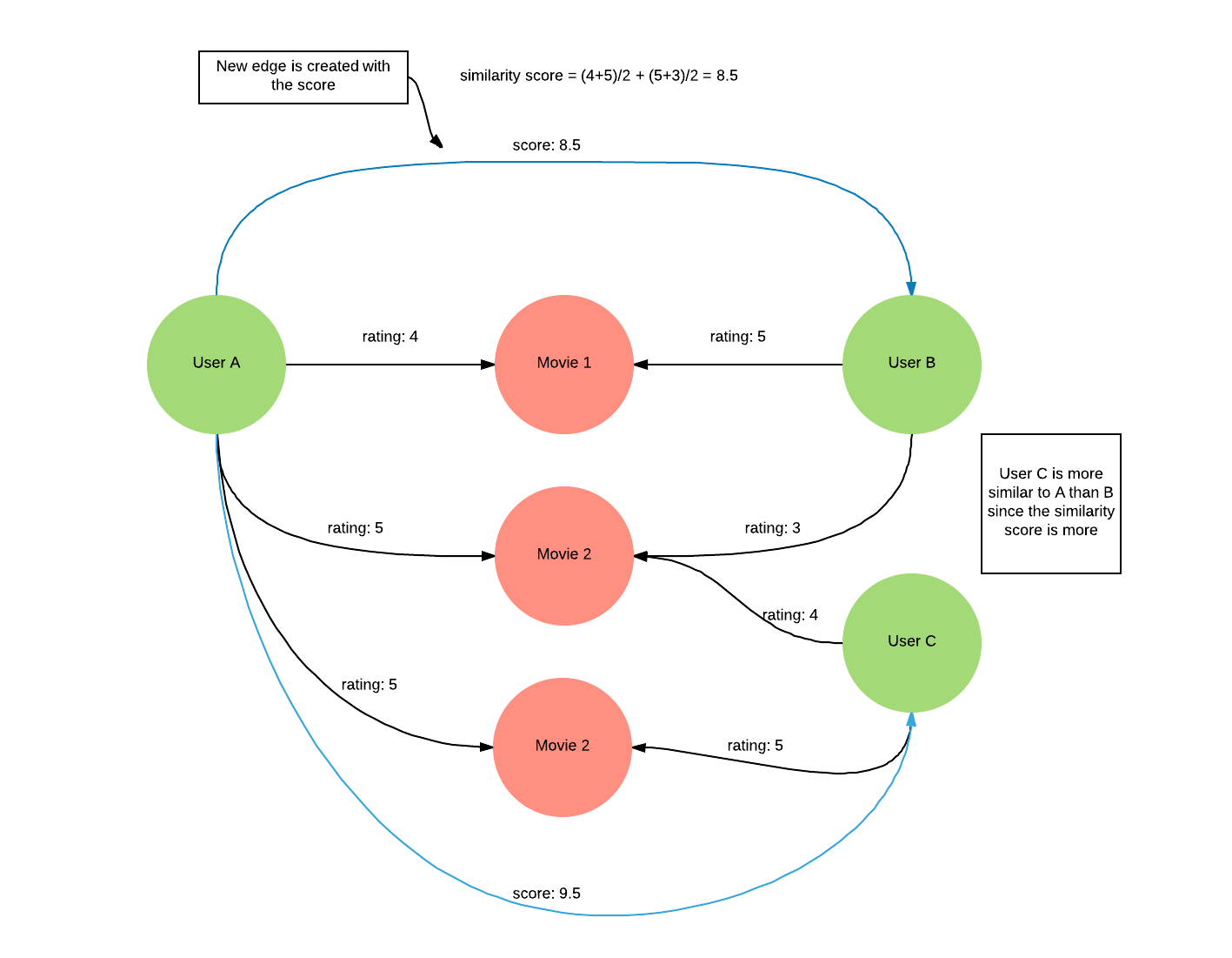
Note that this would require some extra code in the application which creates these edges when an update happens but can make the recommendation query highly performant even for extremely large datasets. Typically user similarity scores are generated as a batch process. With this approach, we can generate these scores incrementally, triggered by user actions; which would also improve the freshness of the recommendations.
Now let’s look at a different kind of dataset which has users, posts (questions, answers, comments), upvotes, downvotes, etc. This has around 450k triples in it and was obtained from Lifehacks Stack Exchange forum.
Say we want to recommend what a user should read based on their upvotes. This is similar to the collaborative filtering we saw in the last section.
First, let’s take a look at the schema for a part of the data that is of interest to us.
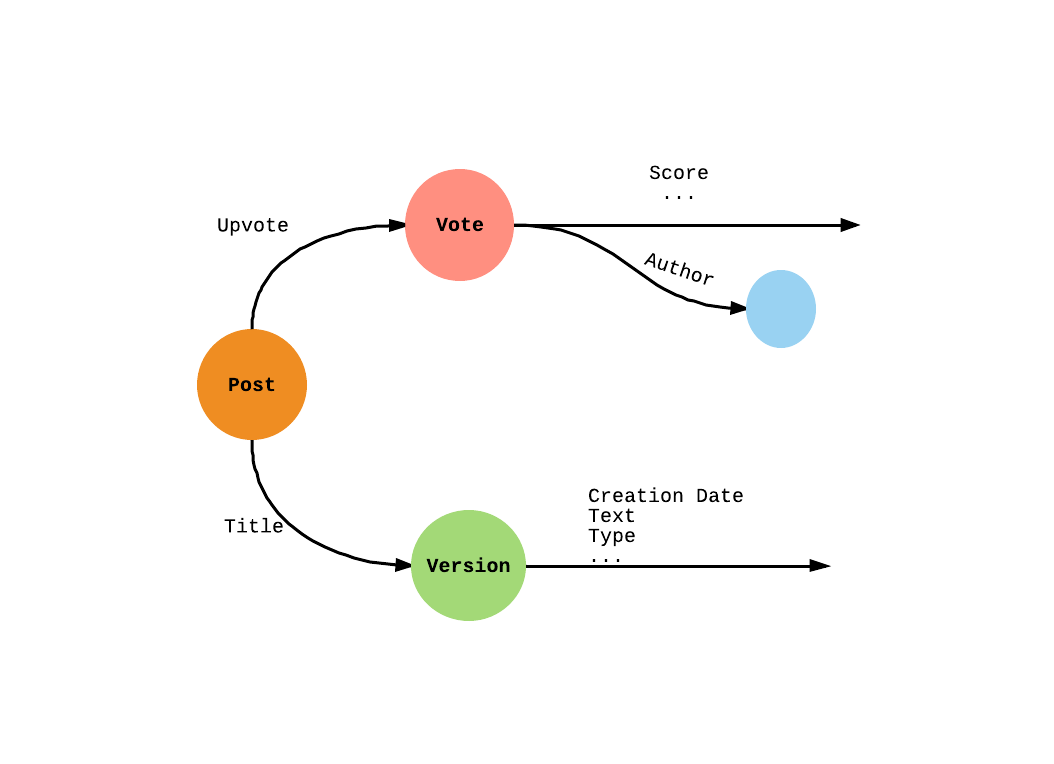
The query to do collaborative filtering on this dataset is as follows:
# Recommend similar questions to read based on upvote.
{
  user as var(func: eq(DisplayName, "Mooseman")) { # 1
    a as math(1)
    ~Author { # 2
      seen as ~Upvote { # 3
        Upvote {    # 4
          Author {  # 5
            sc as math(a)
          }
        }
      }
    }
  }

  var(func: uid(sc), orderdesc: val(sc), first: 50) @filter(not uid(user)) {  # 6
    b as math(1)
    ~Author { # 7
      ~Upvote @filter(not uid(seen) and eq(Type, "Question")) { # 8
        fsc as math(b)
      }
    }
  }

  topQ(func: uid(fsc), orderdesc: val(fsc), first: 10) {  # 9
    Title {
      Text
    }
  }
}
Let’s look at what the numbered lines in the query represent:
Mooseman~Author edge which leads to the votes he has created~Upvote edge which leads us to the posts he has upvotedUpvote edge to get all the upvotes on these postsAuthor edge to get the users who created these upvotes and store the number of paths between the starting user and this user in a variable scMooseman and assign them a score which is the number of upvotes by these top (similar) users. This score is store in variable fscfsc to get the top 10 questionsOutput:
{
  "topQ": [
    {
      "Title": [
        {
          "Text": "How can I keep my cat off my keyboard?"
        }
      ]
    },
    {
      "Title": [
        {
          "Text": "How do I stop my earphones from getting tangled"
        }
      ]
    },
    {
      "Title": [
        {
          "Text": "Ηow can I keep my jeans' zippers from unzipping on their own?"
        }
      ]
    },
    {
      "Title": [
        {
          "Text": "How can I work out my girlfriend's ring size, without asking her or using a ring?"
        }
      ]
    },
    {
      "Title": [
        {
          "Text": "How can I improvise a magnifying glass?"
        }
      ]
    },
    {
      "Title": [
        {
          "Text": "Sleeping in a noisy environment"
        }
      ]
    },
    {
      "Title": [
        {
          "Text": "How can I black out a bright bedroom at night?"
        }
      ]
    },
    {
      "Title": [
        {
          "Text": "How do I stop cars from tailgating?"
        }
      ]
    },
    {
      "Title": [
        {
          "Text": "Driving into garage where there is little room for error?"
        }
      ]
    },
    {
      "Title": [
        {
          "Text": "How can I boost my wifi range?"
        }
      ]
    }
  ]
}
To make this recommendation scalable, we can create an edge between the most similar users when an update (in this case, an upvote) happens. Then, when a user logs in, we can cheaply compute their recommendations using these edges directly.
With that, we conclude this post. In this post, we showed how collaborative filtering based on similar users can be encoded in Dgraph queries. We showed a couple of approaches so you can get a flavour of the kind of flexibility Dgraph allows. We also combined content-based and collaborative approaches into a hybrid recommendation system that found similar users and then ranked movies with genres our user enjoyed.
Content-based filtering can be useful when recommending to users who have rated few movies. This is how websites bootstrap recommendation when you join, for example, by asking for your 5 favourite movies and then showing movies that are similar to them. Then, as you start rating movies, a switch to collaborative filtering utilizes user similarity and starts to improve recommendations further.
We can’t tell you what metrics will work best in your case — that’ll be based on your data and users and a fair amount of thinking and experimenting. But what we’ve done here is to show you how you can translate your ideas into reality using Dgraph. Hope this gets you started on the path to adding a recommendation system in your application.
Watch out for an upcoming series of posts where we explore how typical web apps can benefit from Dgraph. We’ll show how we loaded all the data from the Stack Overflow data dumps, which is more than 2 billion edges, into Dgraph and run Stack Overflow with Dgraph as the sole backend DB. We’ll explore the tradeoffs that are made in doing this in SQL vs a graph database and we’ll look at the recommendation engine we’re building on top of all that Stack Overflow data.