Making Dgraph a truly GraphQL-native database

Choosing between GraphQL vs DQL for your app? Preferring DQL’s speed over GraphQL’s easiness? Wait, GraphQL is as fast as DQL now! Read on to find out more.

But, before we begin, let’s briefly look at what we’ll cover:

• Overview of the initial GraphQL implementation
• Benchmarks to evaluate the GraphQL performance
• Optimizing JSON generation
• Comparison of post-optimization benchmarks
• How JSON generation works within Dgraph?
• Conclusion

Overview of the initial GraphQL implementation

A long time ago in a galaxy far, far away….

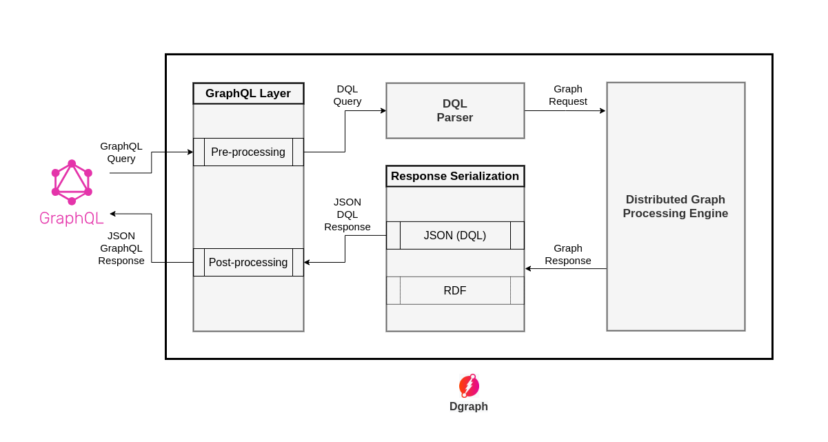
There was once a version of Dgraph without GraphQL. Then, a year ago, we developed an initial implementation of the GraphQL spec. To begin with, we designed it as a simple layer within Dgraph. When hit by a GraphQL query, this layer would execute the following pipeline:

1. Pre-processing
   • Parse the GraphQL query
   • Rewrite the parsed GraphQL query to a DQL query
2. Execution: Run the DQL query within Dgraph
3. Post-processing
   • Unmarshal the DQL formatted JSON response
   • Format the unmarshalled response as per the GraphQL spec requirements
   • Marshal the GraphQL formatted JSON response

The below figure illustrates the same process:

Benchmarks to evaluate the GraphQL performance

By the mid of 2020, we wanted to know how performant was the layer we designed. So, we thought of benchmarking it with GraphQL queries. Benchmarking required a dataset, a GraphQL schema to represent that data, and GraphQL queries to benchmark against. Thanks to Kaggle, we found a publicly available restaurant dataset and created the following schema to represent it:

type Country {
	cid: ID!
	id: String! @id
	name: String!
	cities: [City]
}

type City {
	cid: ID!
	id: String! @id
	name: String!
	country: Country! @hasInverse(field: cities)
	restaurants: [RestaurantAddress] @hasInverse(field: city)
}

interface Location {
	id: ID!
	lat: Float!
	long: Float!
	address: String!
	locality: String!
	city: City!
	zipcode: Int
}

type RestaurantAddress implements Location {
	restaurant: Restaurant! @hasInverse(field: addr)
}

type Restaurant {
	id: ID!
	xid: String! @id
	name: String!
	pic: String
	addr: RestaurantAddress!
	rating: Float
	costFor2: Float
	currency: String
	cuisines: [Cuisine]
	dishes: [Dish] @hasInverse(field: servedBy)
	createdAt: DateTime!
}

type Cuisine {
	id: ID!
	name: String! @id
	restaurants: [Restaurant] @hasInverse(field: cuisines)
	dishes: [Dish] @hasInverse(field: cuisine)
}

type Dish {
	id: ID!
	name: String!
	pic: String
	price: Float!
	description: String
	isVeg: Boolean!
	cuisine: Cuisine
	servedBy: Restaurant!
}

Then, loaded this schema and data into Dgraph using the GraphQL API. Once loaded, this database spanned 74 cities across 15 countries with 8422 restaurants serving 4158700 dishes from 116 different cuisines. So many dishes, I just hope, I can taste them all one day. 😋

As the database was ready, we needed some queries to benchmark it. With queries, we wanted to know how a small change in the query affects the overall latency, and also the time spent exclusively in the GraphQL layer. So, we figured that we would need queries that could vary over the following points:

1. number of data levels in the query
2. number of fields at each level
3. order of traversal
4. response size

Keeping these points in consideration, we designed a set of queries. Let’s take a brief look at one of those queries:

query {
	queryCuisine {
		id
		name
		restaurants {
			name
			rating
		}
	}
}

This query fetches 2 levels of data, with the order of traversal as Cuisine(C)->Restaurant(R). At level-1 it fetches 3 fields (id, name, restaurants) and at level-2 it fetches 2 fields (name, rating). The JSON response to this query is ~744 KiB in size and contains ~17k nodes (116 at level-1 and 16984 at level-2).

The below table contains these details about each query in the set of benchmarking queries:

Once the data, schema, and queries were ready, it was time for us to run the benchmarks. The benchmarking process ran each query 10 times. It collected CPU and memory profiles for each run, and measured the average overall latency, along with the latency incurred exclusively in the GraphQL layer. This gave us the following results (sorted in the increasing order of overall latency):

Let me give some visual perspective to these results. As the scale of response size and latency for the first four queries is very small in comparison to the last four, let me create a logarithmic line chart for better visualization, with the x-axis representing the queries in the increasing order of latency.

One thing that was clearly visible from these results was that, as the response size grew, the overall latency started increasing as well, and so did the latency incurred by the GraphQL layer. On average, the GraphQL layer was consuming ~32% of the overall latency. That was huge!

It seemed as if the Millennium Falcon was captured by the Empire, and it couldn’t fly anymore!

So, we set out to find what part of the GraphQL layer was incurring this cost. We started looking at the CPU profiles collected during the benchmarking process and figured that the post-processing step was consuming almost all the time in the GraphQL layer.

As explained earlier, post-processing was a 3-step process:

1. Unmarshal the DQL formatted JSON response
2. Format the unmarshalled response as per the GraphQL spec requirements
3. Marshal the GraphQL formatted JSON response

For unmarshalling and marshalling the JSON, we were using Go’s standard encoding/json package and the map[string]interface{} data type. And, the CPU profiles were showing that it was the JSON unmarshal/marshal that was incurring this cost in the GraphQL layer.

Optimizing JSON generation

Jedi had to come to rescue the falcon…

GraphQL layer consuming ~32% of the overall latency presented us with an opportunity to iterate and improvise on our initial implementation.

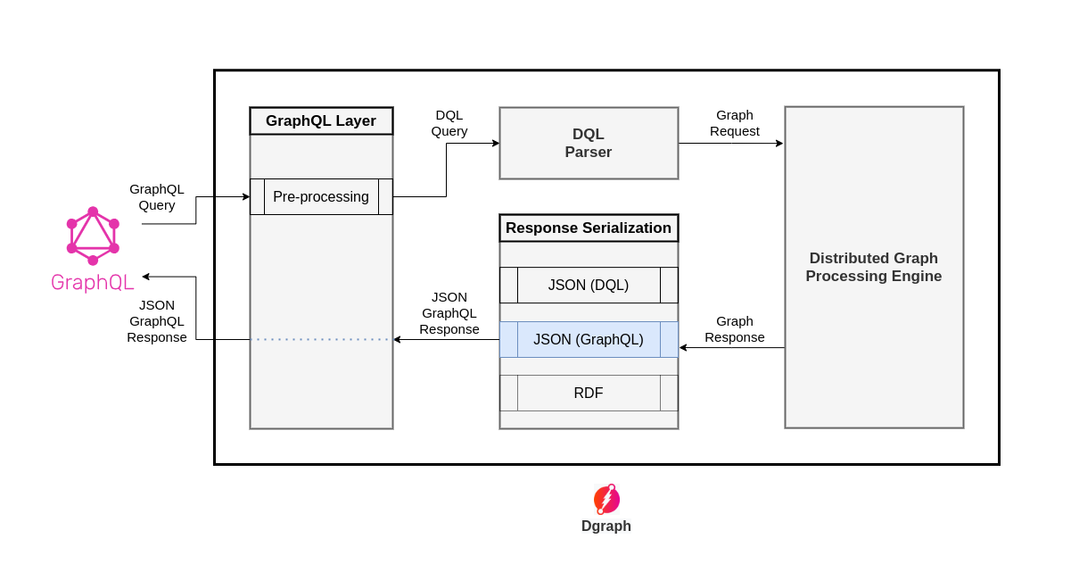
We figured that the post-processing step was unnecessary in the end-to-end query execution pipeline. Instead of first generating a DQL formatted JSON response, and then the GraphQL layer doing the post-processing on that response, we could have directly generated a GraphQL formatted JSON response, and then there would be no post-processing required in the GraphQL layer.

So, we came up with the following new design of the implementation:

Comparison of post-optimization benchmarks

So, we did the above optimization, then benchmarked the same queries on the same dataset, and observed the following results (sorted in the increasing order of overall latency):

Let me show this data again in a logarithmic line chart for better visualization:

Also, let me tell you one thing, the Falcon went warp speed after this rescue operation. 🚀

Comparing the results after the optimization to the ones before, we can make the following observations:

• Overall Latency: We can see that the overall latency has dropped after the optimization. In total, Dgraph now takes 63.25 secs less for querying 971 MiB of data. On a totalistic average, that amounts to a ~33% reduction in overall query latency. This one-third improvement in the query latency also improves the memory utilization, as the memory that was being consumed previously during post-processing would now no more be used.
• GraphQL Latency: From the above graphs, it is visible that after the optimization, the latency incurred solely because of the GraphQL layer is nothing as compared to the pre-optimization scenario. In fact, on a totalistic average, there is a 99.72% drop in the GraphQL latency.
• % GraphQL Latency: It is visible that out of the total query execution time, the % of latency incurred by the GraphQL layer is less than 1% for all the queries with big response sizes. And, on a totalistic average, it has significantly dropped to ~0.13% from ~32%. This means that GraphQL queries now perform almost the same as DQL queries, with avg latency overhead of only 0.13%.
• Small-sized queries: For queries with small response sizes (like 00.query), the latency drop (although ~13% overall and 61% in the GraphQL layer) isn’t as significant as compared to the queries with large response sizes. It is because the optimization is highly correlated with the response size. It only removes the latency incurred because of the large JSON response. So, as the response size decreases, the effects of the optimization start diminishing because other things like query parsing still consume a constant amount of time.

Cool! So how does JSON generation work within Dgraph?

Not so easy! Do you know what powers the Falcon?

Quadex Power Core, and 3 droid brains, they say. 😉

But really, how does Dgraph efficiently encode a Graph response to JSON?

Internally, we don’t use Go’s default encoding/json package for this. We have built our own custom encoder, specifically to convert a Graph response to JSON. This encoder is packed with lots of memory optimizations. I won’t go into the complete details of it, but here is a high-level overview of what it does:

• Visualize the JSON as a tree. Where a node in the tree represents a key-value pair, with the leaf nodes representing the scalar key-value pairs. We call this tree, the fastJson tree and a node in this tree as a fastJsonNode. As a first step, we construct this tree from a Graph response.

• A fastJsonNode doesn’t store the key and the value directly. Otherwise, that would lead to high memory fragmentation. Instead, it stores only 3 pieces of information:

  • meta: a uint64 that stores various kinds of information at the byte level.
  • next: a pointer to the next sibling of this node.
  • child: a pointer to the first child of this node, if this node wasn’t a scalar.

• Now, Given a JSON like this:

  {
    "q": [
      {"k1": "v1.1", "k2": "v2.1", "k3": true},
      {"k1": "v1.2", "k2": "v2.2", "k3": true},
      ...
      {"k1": "v1.n", "k2": "v2.n", "k3": true}
    ]
  }
  

  We can see that the keys remain the same for all objects, it is just the value that changes. So, there is no point in allocating new space for the same key string every time it is encountered in a new object. Instead, we assign each unique key a unique 16-bit integer (called attrId) and store only the attrId in 2 specific bytes of the fastJsonNode’s meta.

• For storing the scalar values, we allocate one large byte buffer, called the arena, and store the values in the arena. That again helps avoid memory fragmentation. In 4 specific bytes of the fastJsonNode’s meta, we store the offset of the value in the arena.

• Another optimization is that if a scalar value repeats in the JSON, then there is no point storing it twice in the arena and wasting memory. For example, the boolean value true might repeat itself across a lot of JSON objects. For tackling such cases, we maintain a map from the hash of the value to its offset in the arena, so while inserting a new value we can figure out if the value already exists in the arena or not, and return the offset accordingly.

• Finally, we have a recursive algorithm to encode the whole fastJson tree to one large byte buffer, which represents the raw JSON response that would be sent to the user.

All of this might sound a bit too technical, but this is what powers the JSON encoding!

Conclusion

From a time of no GraphQL support, to supporting GraphQL natively with as good speed as DQL, Dgraph has improved a lot in the past year. If you compare the v21.03 release with the v20.03 release, you would find that your GraphQL queries are magically ~33% faster. The GraphQL layer is now just a thin wrapper around the core of Dgraph, and we are happy to say that Dgraph is now a truly GraphQL-native database.

We believe that as a user of a Graph database, the performance of your queries should not be affected by the choice of the query language. That is what we tried to achieve through this optimization. Now, whether you query with GraphQL or DQL, both perform almost the same. Going forward, we will try to further reduce the 0.13% latency difference between GraphQL and DQL, as the queries which return small-sized response will greatly benefit from it. That’s my promise for a future blog post.

Stay tuned!